Project 1: Orientation Tracking and Panorama Construction
Orientation Estimation
The problem is be formulated as follows: given measurements of the IMU’s angular velocity \(\boldsymbol{\omega}_t\) and linear acceleration \(\mathbf{a}_t\) over time, estimate the body’s orientation at time \(t\) using a unit quaternion \(q_t \in \mathbb{H}^*\). To achieve this, a motion model and an observation model are needed to define a cost function.
Motion Model
Estimating the quaternion at the subsequent step \(q_{t+1}\) can be accomplished by using the IMU angular velocity measurements \(\boldsymbol{\omega}_t\) and the differences between consecutive time stamps \(\tau_t\). This is achieved through the following kinematic motion model:
\[
q_{t+1} = f(q_t, \tau_t \boldsymbol{\omega}_t) := q_t \circ \exp\left(\frac{1}{2} [0, \tau_t \boldsymbol{\omega}_t]\right) \tag{1}
\]
In Equation (1), the function \(f(q_t, \tau_t \boldsymbol{\omega}_t)\) represents the motion model. \(q_{t+1}\) represents the quaternion at the subsequent step, and \(q_t\) denotes the quaternion at the current step. \(\tau_t \boldsymbol{\omega}_t\) represents the product of the time difference between consecutive timestamps \(\tau_t\) and the IMU’s angular velocity \(\boldsymbol{\omega}_t\). The term \(\exp\left(\frac{1}{2} [0, \tau_t \boldsymbol{\omega}_t]\right)\) denotes the quaternion exponential of the scaled rotation increment \(\frac{1}{2} [0, \tau_t \boldsymbol{\omega}_t]\), and \(\circ\) denotes quaternion multiplication.
Observation Model
Because the body undergoes pure rotation, the acceleration of the body is approximately \([0, 0, -g]\) in the world frame of reference, with \(g\) denoting the gravitational acceleration. Therefore, the measured acceleration \(\mathbf{a}_t\) in the IMU frame should align with the gravitational acceleration after transformation to the IMU frame using the orientation \(q_t\), resulting in the following observation model:
\[
\mathbf{a}_t = h(q_t) := q_t^{-1} \circ [0, 0, 0, -g] \circ q_t \tag{2}
\]
In Equation (2), \(\mathbf{a}_t\) represents the measured acceleration in the IMU frame. The function \(h(q_t)\) denotes the observation model, where \(q_t^{-1}\) represents the inverse of the quaternion \(q_t\). The term \([0, 0, 0, -g]\) denotes the acceleration due to gravity in the IMU frame, with an additional zero appended at the beginning of the vector to enable quaternion multiplication.
Cost Function
With the motion model and the observation model, an optimization problem can be formulated to estimate the orientation trajectory \(q_{1:T} = \{q_1, q_2, \ldots, q_T\}\). The cost function for the optimization problem can be defined as:
\[
c(q_{1:T}) := \frac{1}{2} \sum_{t=0}^{T-1} \left\| 2 \log \left( q_{t+1}^{-1} \circ f(q_t, \tau_t \boldsymbol{\omega}_t) \right) \right\|^2 + \frac{1}{2} \sum_{t=1}^{T} \left\| \mathbf{a}_t – h(q_t) \right\|^2 \tag{3}
\]
In Equation (3), the cost function \(c(q_{1:T})\) is composed of two terms. The first term, \(\frac{1}{2} \sum_{t=0}^{T-1} \left\| \log \left( q_{t+1}^{-1} \circ f(q_t, \tau_t \boldsymbol{\omega}_t) \right) \right\|^2\), represents the difference between the estimated orientations \(q_{t+1}\) and the motion model prediction \(f(q_t, \tau_t \boldsymbol{\omega}_t)\) over the trajectory \(q_{1:T}\). The logarithm function is used to convert the quaternion difference into a vector that can be squared and summed to form part of the cost function. The second term, \(\frac{1}{2} \sum_{t=1}^{T} \left\| \mathbf{a}_t – h(q_t) \right\|^2\), represents the difference between the measured accelerations \(\mathbf{a}_t\) and the predicted accelerations \(h(q_t)\) over the trajectory \(q_{1:T}\).
Constrained Optimization
With the cost function defined and the quaternions \(q_t\) required to maintain a unit norm, i.e., \(q_t \in \mathbb{H}^*\), throughout the optimization process to accurately represent orientations and rotations, a constrained optimization problem is formulated as follows:
\[
\text{minimize} \quad c(q_{1:T})
\]
\[
\text{subject to} \quad \|q_t\|^2 = 1, \quad \forall t \in \{1, 2, \ldots, T\}
\]
This formulation ensures that each quaternion \(q_t\) remains a unit quaternion throughout the optimization process.
Projected Gradient Descent
To minimize the cost function \( c(q_{1:T}) \), gradient descent is employed. The aim is to iteratively update the quaternions matrix \( q_{1:T} \) in the direction of the steepest descent of the cost function. The gradient descent equations for updating the quaternions \( q_{1:T} \) at each iteration \( t \) are as follows:
\[
q_{1:T}^{(t+1)} := q_{1:T}^{(t)} – \alpha \left( \nabla c(q_{1:T}) \right) \tag{4}
\]
Here, \( \alpha \) denotes the learning rate, which determines the size of the steps taken in the parameter space during each iteration. A higher learning rate results in larger steps, potentially leading to faster convergence but risking overshooting the optimal solution. Conversely, a lower learning rate may lead to slower convergence but with more stable progress. For this project, it is chosen to be 0.13 by trial and error. The initial \( q_{1:T}^{(t)} \) is determined by performing quaternion integration on an identity quaternion using the angular velocities obtained from the IMU.
After calculating the next step, the quaternions \( q_{1:T}^{(t+1)} \) are normalized to satisfy the constraints:
\[
q_{1:T}^{(t+1)} = \frac{q_{1:T}^{(t+1)}}{\|q_{1:T}^{(t+1)}\|} \tag{5}
\]
It is worth mentioning that before taking the logarithm of the quaternion, an extremely small value is added to the quaternion to ensure numerical stability and prevent issues such as division by zero or taking the logarithm of zero, which can lead to undefined or erroneous results.
Results
Below are the Euler angles from the projected gradient descent algorithm and the ground truth for different datasets.
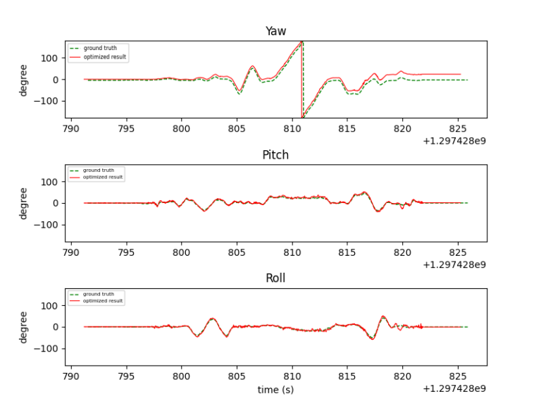
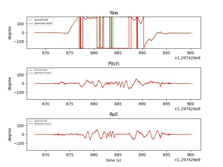
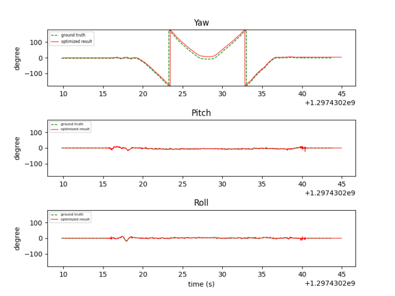
From the plotted data, it’s evident that the estimated roll and pitch angles (red lines) closely match the ground truth values (green dotted lines), demonstrating a high level of agreement. However, the yaw angle estimation, while generally close to the ground truth, does not exhibit the same level of accuracy as the roll and pitch angles. This discrepancy arises because the accelerometer only provides information about the roll and pitch angles, not the yaw angle. Consequently, the estimation of the yaw angle relies solely on the gyroscope readings, which are prone to gyro drifting over time. To mitigate this issue, incorporating a magnetometer into the sensor fusion process could help improve the accuracy of the yaw angle estimation by providing additional information about the orientation relative to the Earth’s magnetic field.
Panorama Construction
With the estimated orientations and the given images, a panorama can be constructed. This process involves mapping each pixel of the image, assumed to be projected onto a unit spherical surface, to its corresponding world coordinates:
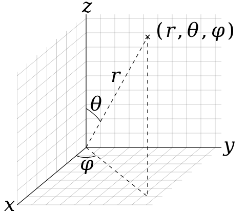
1. Find longitude (\(\phi\)) and latitude (\(\theta\)) of each pixel: Using the number of rows and columns in the image and the horizontal (60°) and vertical (45°) fields of view, compute the longitude and latitude values for each pixel. These values determine the angular position of each pixel on the spherical surface.
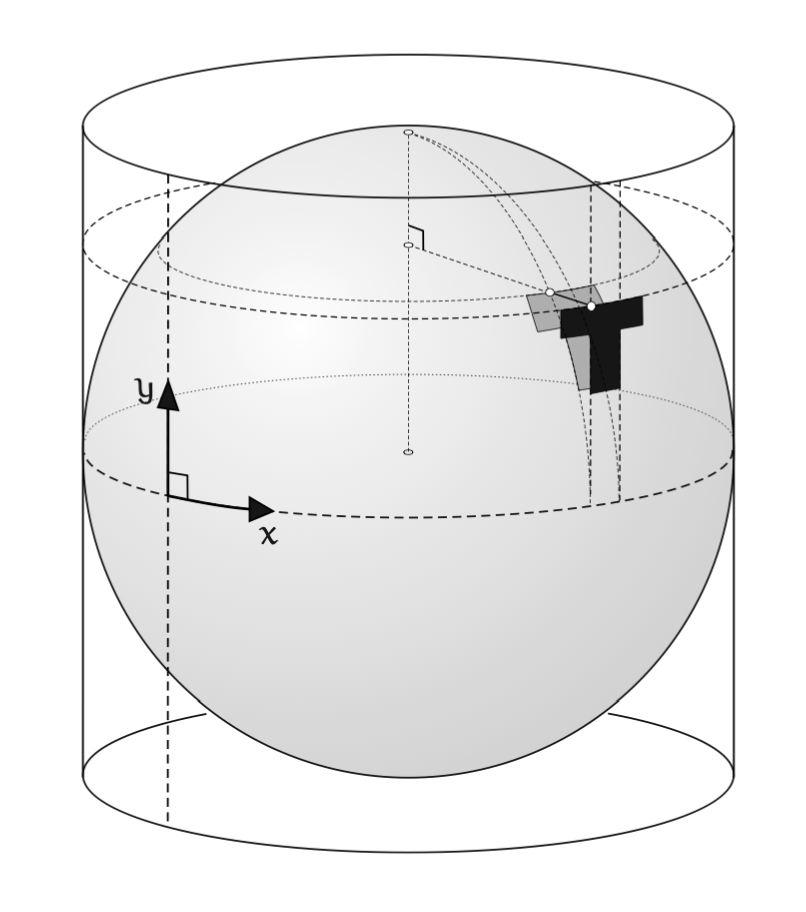
2. Convert spherical (\(\phi, \theta, 1\)) to Cartesian coordinates (Fig. 1): Once the longitude and latitude of each pixel are determined, convert these spherical coordinates to Cartesian coordinates assuming a depth of 1. This transformation maps each pixel’s angular position to a point in 3D space.
3. Rotate the Cartesian coordinates to the world frame using \(R\): Apply a rotation matrix \(R\), which is obtained from the estimated orientation, to the Cartesian coordinates of each pixel to align them with the world frame. This step ensures that the coordinates of the pixels are adjusted to match the orientation of the environment captured by the camera.
4. Convert Cartesian back to spherical coordinates: Transform the rotated Cartesian coordinates of each pixel to spherical coordinates. This step is crucial for the subsequent projection onto a cylinder.
5. Inscribe the sphere in a cylinder: Place the sphere within a cylinder so that each point \((\phi, \theta, 1)\) on the sphere corresponds to a height of \(\theta\) on the cylinder and a longitude of \(\phi\) along the circumference of the cylinder (Fig. 2).
6. Unwrap the cylinder surface to a rectangular image: Flatten out the surface of the cylinder to create a rectangular image with a width of \(2\pi\) radians and a height of \(\pi\) radians. In this project, the resolution of the final panorama is chosen to be 1000 pixels (vertical) by 2000 pixels (horizontal).
Results
Below are the panoramas generated using the estimated orientations obtained from the preceding part of the project.
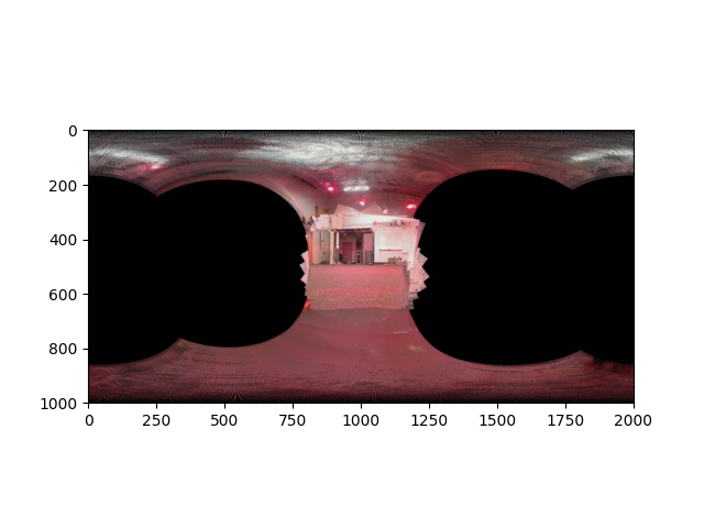
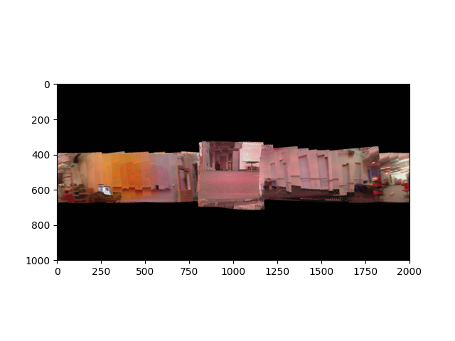
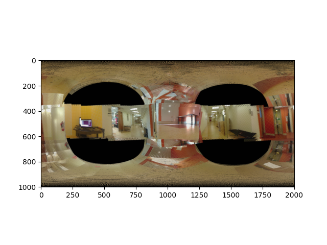
From the analysis of the panoramas, it is evident that the overall quality of the final stitched images is satisfactory, with clear representations of the captured scenes. However, some distortions are observed, primarily attributed to inaccuracies in the orientation estimation.