Project 2: LiDAR-Based Simultaneous Localization and Mapping (SLAM)
In this project, for the localization step, data from an encoder and an IMU (Inertial Measurement Unit) from a differential-drive robot are used along with the Euler method of integration for an initial guess of the trajectory of a differential-drive robot. Then, data from a 2-D LiDAR scanner and Iterative Closest Point (ICP) algorithm, Kabsch algorithm, and loop closure and pose graph optimization are utilized to improve the accuracy of the trajectory. Additionally, LiDAR measurements are used to construct occupancy grid maps, and RGBD camera images are used to construct texture maps representing the environment surrounding the robot, forming the mapping step in SLAM.
Localization
Differential-Drive Kinematic Model
For differential drive systems, the motion of the system can be described using the following differential equations:
\[
\dot{x} = v \cdot \cos(\theta)
\]
\[
\dot{y} = v \cdot \sin(\theta)
\]
\[
\dot{\theta} = \omega
\]
Where:
– \(x\) and \(y\) are the positions in the horizontal and vertical axes, respectively.
– \(\theta\) is the orientation angle of the robot with respect to the world frame.
– \(v\) is the linear velocity of the robot.
– \(\omega\) is the angular velocity of the robot.
Euler integration is a numerical method used to approximate the solution of ordinary differential equations (ODEs). In Euler integration, time is discretized into small intervals, denoted by \(\Delta t\). Then, the derivatives are approximated in the above equations using finite differences. The discrete equations for Euler integration become:
\[
x_{t+1} = x_t + v_t \cdot \cos(\theta_t) \cdot \Delta t
\]
\[
y_{t+1} = y_t + v_t \cdot \sin(\theta_t) \cdot \Delta t
\]
\[
\theta_{t+1} = \theta_t + \omega_t \cdot \Delta t
\]
Where:
– \(x_t\), \(y_t\), and \(\theta_t\) are the values of \(x\), \(y\), and \(\theta\) at time step \(t\), respectively.
– \(v_t\) and \(\omega_t\) are the values of linear and angular velocities at time step \(t\), respectively.
In this project, these equations are used to represent the update rules for the position and orientation of the robot at each time step using Euler integration.
Iterative Closest Point (ICP) Algorithm
Given two sets of 3D points \( A = \{ \mathbf{a}_1, \mathbf{a}_2, \ldots, \mathbf{a}_n \} \) and \( B = \{ \mathbf{b}_1, \mathbf{b}_2, \ldots, \mathbf{b}_n \} \), where the correspondence between points in set \( A \) and set \( B \) is unknown, the task is to find the optimal rigid transformation (rotation and translation) that aligns the points in set \( A \) to the points in set \( B \). This alignment should minimize the Root Mean Squared Error (RMSE) between corresponding points.
The steps of the ICP algorithm with the Kabsch algorithm can be summarized as follows:
1. Initialization: Begin with an initial guess for the transformation, which can be obtained from the encoder and IMU motion model.
2. Point Correspondence: Find the closest points in set \( B \) for each point in set \( A \). This step establishes point correspondences \(\Delta = \{(i, j)\}\). This is done using the cKDTree function in Python.
3. Compute Centroids: Calculate the centroids of both sets of points.
\[
\mathbf{c}_A = \frac{1}{n} \sum_{i=1}^{n} \mathbf{a}_i
\]
\[
\mathbf{c}_B = \frac{1}{n} \sum_{j=1}^{n} \mathbf{b}_j
\]
4. Center the Points: Subtract the centroids from each set of points to center them around the origin:
\[
\mathbf{\hat{a}}_i = \mathbf{a}_i\, – \,\mathbf{c}_A
\]
\[
\mathbf{\hat{b}}_j = \mathbf{b}_j\, – \,\mathbf{c}_B
\]
5. Compute Covariance Matrix: Compute the covariance matrix \( Q \) between the centered point sets:
\[
Q = \sum_{i=1}^{n} \mathbf{\hat{b}}_j \,\mathbf{\hat{a}}_i^T
\]
6. Singular Value Decomposition (SVD): Perform Singular Value Decomposition on \( Q \) to obtain \( U \), \( \Sigma \), and \( V^T \).
7. Rotation Matrix \( R \): Calculate the rotation matrix \( R \) using the computed \( U \) and \( V^T \) matrices:
\[
S = \begin{bmatrix} 1 & 0 & 0 \\ 0 & 1 & 0 \\ 0 & 0 & \text{det}(U V^T) \end{bmatrix}
\]
\[
R = U S\, V^T
\]
8. Translation Vector \( t \): Compute the translation vector \( t \) based on the centroids and the rotation matrix \( R \):
\[
\mathbf{t} = \mathbf{c}_B\, – \,R\, \mathbf{c}_A
\]
9. Update Point Cloud, Transformation Matrix, and RMSE: Apply the rotation and translation to point cloud \( A \). Update the transformation matrix \( T \) by multiplying the previous transformation matrix \( T_{n-1} \) with the current transformation \( T_{n} \). Update the RMSE between corresponding points to assess the alignment quality.
10. Check for Convergence: Repeat steps 2-9 until convergence criteria are met (e.g., RMSE less than a threshold, error reduction too small, or a maximum number of iterations reached). Once convergence is achieved, the final transformation matrix \( T \) represents the optimal transformation that aligns the points in set \( A \) to the points in set \( B \).
However, since the ICP algorithm’s performance can heavily depend on the initial guess for the transformation parameters, it’s crucial to explore strategies to improve its robustness. In this project, we can assume that the object only rotates around the \( z \)-axis. The following steps describe the improved ICP algorithm:
1. Assume Rotation Around \( z \)-Axis and Discretize Yaw Angles: Assume rotational motion only around the \( z \)-axis and discretize the possible yaw angles. Initialize rotations accordingly.
2. Perform Multiple ICP Runs: Execute the ICP algorithm multiple times, each with a different initial yaw angle.
3. Evaluate Results Using RMSE: Compute the RMSE of the resulting point clouds for each run.
4. Select Optimal Initial Guess: Determine the optimal initial guess for the yaw angle based on the statistics gathered from the multiple ICP runs. Choose the run with the minimum RMSE as the best result.
This refined approach is chosen in this project to systematically test different initial guesses for the ICP algorithm, leading to improved alignment results by selecting the best transformation.
LiDAR Scan Matching
With the ICP algorithm and the trajectory estimated by the motion model available, LiDAR scan matching can be performed as follows:
1. Conversion to Cartesian Coordinates: Assuming the LiDAR frame is aligned with the robot’s frame, there is only a small amount of translation in the x-axis. Remove points that are too close or too far (less than 0.1m and larger than 30m). Convert the cylindrical coordinates (angle, distance) from each LiDAR scan in the sensor frame to Cartesian coordinates (x, y) in the robot frame to obtain two 2D point clouds representing the environment in consecutive scans:
\[
x = \text{distance} \times \cos(\text{angle}) \,-\, 0.15
\]
\[
y = \text{distance} \times \sin(\text{angle})
\]
2. Initialization with Odometry: Initialize the Iterative Closest Point (ICP) algorithm using the odometry estimated from the motion model (encoder and IMU measurements) and the discretized yaw angles.
3. ICP Algorithm: Apply the ICP algorithm to align the two 2D point clouds and estimate the relative pose change between them. Choose the best transformation from the different ICP runs with different initial yaw rotations.
4. Estimating Robot Pose: Once the relative pose change between consecutive frames \( T_t \) and \( T_{t+1} \) is known, the robot’s pose at time \( t+1 \) (\( T_{t+1} \)) can be approximated as the product of the current pose \( T_t \) and the relative pose change \( {}_{t}T_{t+1} \):
\[
T_{t+1} = T_t \cdot {}_{t}T_{t+1}
\]
This approach is employed in the project to provide a more accurate estimation of the robot’s trajectory. It enhances the precision of trajectory estimation by leveraging the capabilities of the ICP algorithm.
Factor Graph SLAM
GTSAM, or Georgia Tech Smoothing and Mapping, is a software library designed for solving optimization problems in robotics and computer vision. It provides tools for constructing and optimizing factor graphs, which are graphical models representing relationships between variables and measurements. GTSAM is widely used for solving problems related to SLAM, sensor fusion, and pose graph optimization. In this project, given the robot’s trajectory estimated by ICP, further improvement can be made using GTSAM. This project follows the subsequent steps:
1. Constructing the Factor Graph: Initiate the creation of a factor graph by creating nodes to denote the robot’s poses at different time instances. The interconnections among these nodes, or edges, represent the relative poses derived from ICP scan matching. Include a prior factor with the pose (0,0,0) to the first pose of the graph. Furthermore, considering the robot returns close to its initial position, apply ICP to match the first and last LiDAR scans and determine the final pose. Integrate this final pose as an additional prior factor.
2. Add Fixed-interval Loop Closure: After every fixed number of robot poses (e.g., every 9 poses in this project), use the ICP scan matching algorithm to estimate the relative pose between the two LiDAR scans. If the error is smaller than a threshold, then introduce a loop closure constraint by adding an edge in the factor graph.
3. Optimize the Trajectory and Reconstruct Mappings: Utilize the Levenberg-Marquardt optimizer to optimize the factor graph. This optimization process aims to minimize the discrepancy between the measured relative poses and the estimated absolute poses, thereby improving the accuracy of the robot’s trajectory.
Results
Below are the results from running the ICP algorithm on images of the drill and liquid container to evaluate the accuracy and effectiveness of the algorithm.
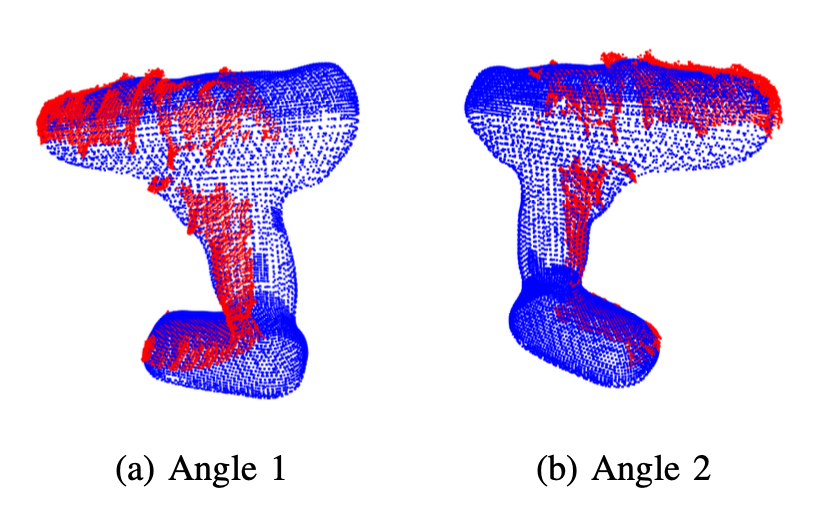
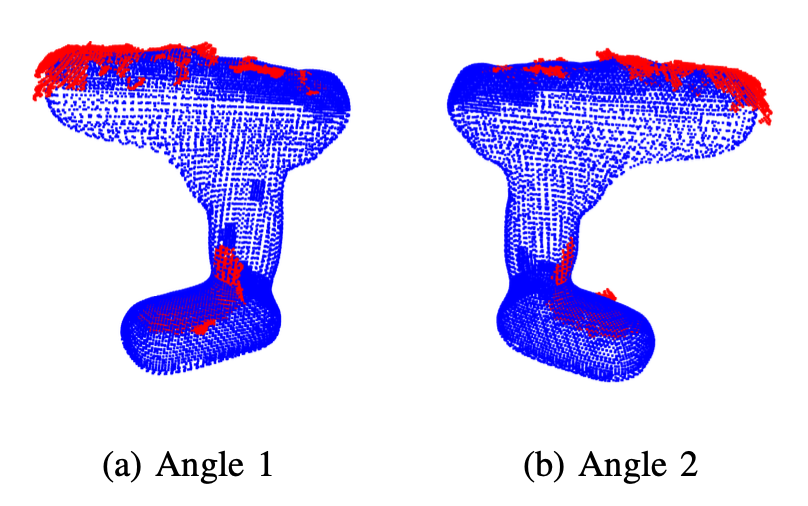
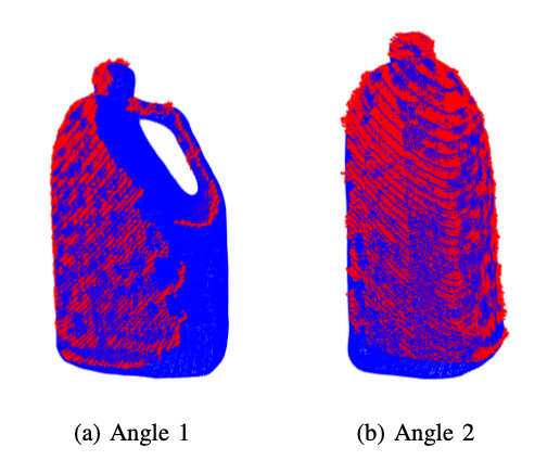
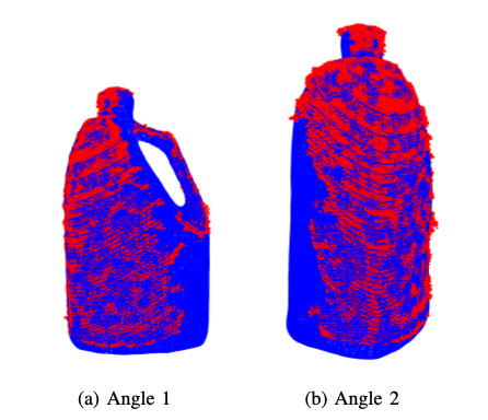
Upon visual inspection, it is evident that the ICP algorithm adeptly determines the transformation required to align the measurement point cloud with the source point cloud for all images of both the drill and the liquid container. The successful alignment observed across all images demonstrates the robustness and reliability of the ICP algorithm in various scenarios, affirming its efficacy.
Below are the trajectories estimated by the motion model, scan matching, and GTSAM.
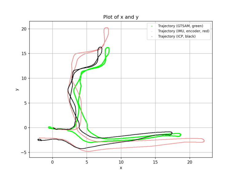
Given the back-and-forth movement of the robot within the hallway, the trajectory comparison (Figure 10 and Figure 17) clearly demonstrates that the trajectory estimated by GTSAM is the most accurate. This determination is based on its minimal trajectory deviation and its provision of a more plausible trajectory estimation compared to other methods. The motion model relying on IMU and encoder data offers an initial trajectory estimate that is reasonable but fails to address accumulating errors over time. Likewise, while ICP can enhance the trajectory estimate to a certain degree, it does not resolve these accumulating errors. However, the integration of loop closure information enables the effective correction of these accumulating errors, leading to a more precise estimation.
Mapping
Occupancy Grid Mapping
Given LiDAR scans and the estimated trajectory of the robot, an occupancy grid map can be created as follows:
1. Transform LiDAR Points to World Frame: Remove points that are too close or too far (less than 0.1m and larger than 30m). LiDAR points are initially in the LiDAR frame. To incorporate these points into the occupancy grid map, they need to be transformed into the world frame.
\[
\begin{bmatrix}
x_{\text{World}} \\
y_{\text{World}} \\
1
\end{bmatrix}
=
{}_{\text{World}}T_{\text{LiDAR}}
\begin{bmatrix}
x_{\text{Lidar}} \\
y_{\text{Lidar}} \\
1
\end{bmatrix}
\]
\[
{}_{\text{World}}T_{\text{LiDAR}} = {}_{\text{World}}T_{\text{Robot}} \ {}_{\text{Robot}}T_{\text{LiDAR}}
\]
\[
{}_{\text{World}}T_{\text{Robot}} =
\begin{bmatrix}
\cos(\theta) & -\sin(\theta) & x \\
\sin(\theta) & \cos(\theta) & y \\
0 & 0 & 1
\end{bmatrix}
\]
\[
{}_{\text{Robot}}T_{\text{LiDAR}} =
\begin{bmatrix}
1 & 0 & 0.15 \\
0 & 1 & 0 \\
0 & 0 & 1
\end{bmatrix}
\]
where:
– \( \theta \) is the orientation angle of the robot in the world frame.
– \( (x, y) \) represents the position of the robot in the world frame.
2. Bresenham’s line algorithm for Occupied and Free Cells: Bresenham’s line algorithm (bresenham2D) is utilized to determine the set of cells (both occupied and free) within the occupancy grid map corresponding to the LiDAR scan. Cells intersected by the LiDAR scan endpoints are considered occupied, while those traversed by the LiDAR scan are deemed free.
3. Update Log-Odds in Occupancy Grid Map: The occupancy grid map is represented using log-odds, where each cell stores a log-odds value indicating the probability of occupancy. This value is updated based on the LiDAR scan data:
\[
\text{log_odds}_{\text{new}} = \text{log_odds}_{\text{old}} + \log(9) \quad \text{(occupied cells)}
\]
\[
\text{log_odds}_{\text{new}} = \text{log_odds}_{\text{old}}\, – \log(9) \quad \text{(free cells)}
\]
Additionally, the values of \( \text{log_odds}_{\text{new}} \) are clipped between \( -40 \log(9) \) and \( 40 \log(9) \) to avoid overconfident estimations.
4. Repeat for Each LiDAR Scan: Apply the same procedure to the entire robot trajectory estimated by the ICP algorithm to generate a complete occupancy grid map of the environment.
5. Convert Log-Odds to Probability: After finalizing the map, convert the log-odds back to probabilities of occupancy using the formula:
\[
p = \frac{e^{\text{log_odds}}}{1 + e^{\text{log_odds}}}
\]
These steps are used in this project to generate an occupancy grid map based on the robot’s trajectory and LiDAR scans, effectively creating a representation of the environment.
Texture Grid Mapping
Given RGBD images captured by the RGBD camera and the estimated trajectory of the robot, a texture map can be created as follows:
1. SLAM Pose Matching: Given the irregular timing of the Kinect camera data, determine the closest SLAM pose that matches the timestamp of the current Kinect scan.
2. Depth Extraction: Given the values \( d \) at pixel \((i,j)\) of the disparity image, extract the depth information.
3. Coordinate Transformation: Transform the coordinates of the pixels in the image frame to the world frame.
4. Plane Identification: Identify the plane corresponding to the occupancy grid in the transformed data. This is achieved by thresholding on the height, where a height of 0 meters indicates the floor plane. The threshold is chosen to be 0.3m.
5. Texture Map Generation: Create a second map (RGB image) with the same resolution as the occupancy grid. Color the pixel coordinates of \((x_w, y_w)\) based on the pixel location of the associated RGB color, which can be calculated from the image data.
Results
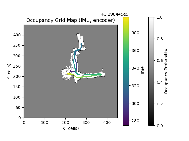
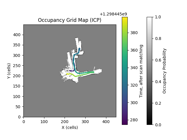
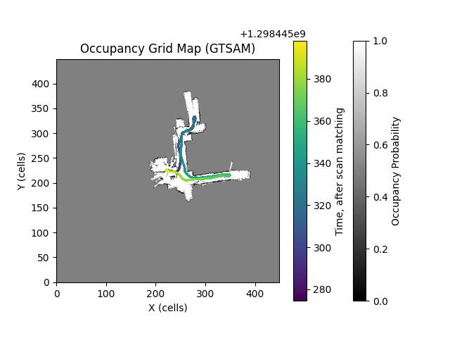
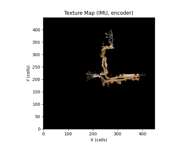
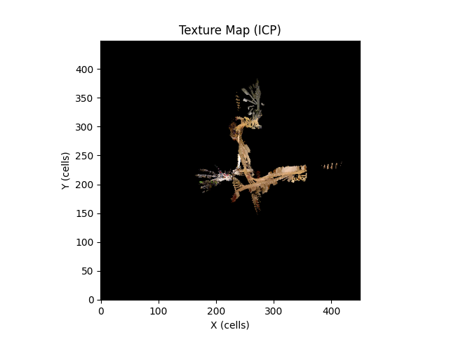
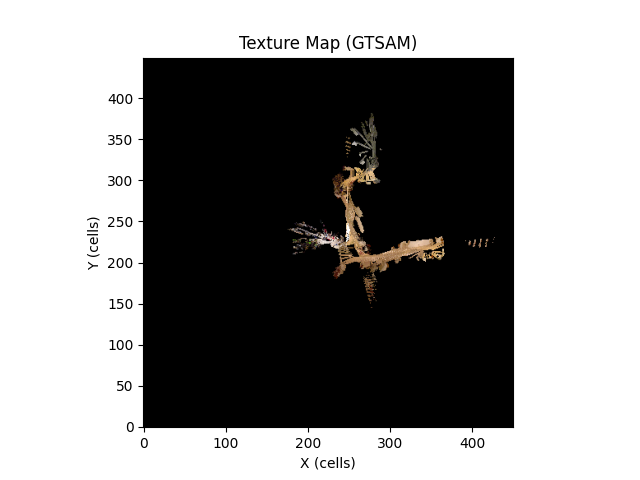
Displayed below are the occupancy grid maps and texture maps corresponding to the trajectories estimated by each algorithm.
It is evident that the occupancy map constructed from the GTSAM-optimized trajectory provides the most accurate representation of the hallway. This conclusion is supported by the minimal overlap and the close resemblance of the map to real-life hallway layouts, compared to the other generated maps. The reduced overlap indicates a more precise mapping of occupied and free spaces, resulting in a clearer depiction of the environment.
While it may be challenging to definitively determine the most accurate texture map due to their similar appearances, the superior trajectory estimation and occupancy grid map produced by the GTSAM algorithm suggest that the texture map generated using the GTSAM-optimized trajectory is the most reliable among the three options.
