Project 3: Visual-Inertial Simultaneous Localization and Mapping (SLAM)
This project aims to tackle the visual-inertial SLAM problem using data from an Inertial Measurement Unit (IMU) and a stereo camera. In the first part, only IMU data are used to provide an initial estimate of the vehicle’s trajectory. Subsequently, data from both the IMU and stereo camera are combined to perform a complete visual-inertial SLAM algorithm, employing an Extended Kalman Filter (EKF) to estimate the vehicle’s trajectory and the positions of landmarks. The results highlight the sensitivity of the estimated trajectory to noise levels and the number of feature points used, emphasizing the importance of accurately estimating noise values and filtering out poor feature points.
Technical Approach
IMU Localization
Given linear velocity \( \mathbf{v}_t \) and rotational velocity \( \boldsymbol{\omega}_t \) of the IMU, the IMU pose at time \( t+1 \) can be estimated using the motion model:
\[
T_{t+1} = T_t \cdot \exp(\tau_t \hat{\xi}_t)
\]
where \( \hat{\xi}_t \) is the skew-symmetric matrix of the twist vector \( \xi_t = [\mathbf{v}_t, \boldsymbol{\omega}_t]^T \). The skew-symmetric matrix \( \hat{\xi}_t \) is given by:
\[
\hat{\xi}_t = \begin{bmatrix}
0 & -\omega_{z,t} & \omega_{y,t} & v_{x,t} \\
\omega_{z,t} & 0 & -\omega_{x,t} & v_{y,t} \\
-\omega_{y,t} & \omega_{x,t} & 0 & v_{z,t} \\
0 & 0 & 0 & 0 \\
\end{bmatrix}
\]
Starting with an identity matrix, perform this operation for all time steps, and an estimation of the IMU trajectory can be obtained.
Landmark Mapping
Assuming the predicted IMU trajectory \( {}_{\text{W}}T_{\text{I}} \) is given, along with camera data (the left and right image pixels of the features over time \( \mathbf{z}_{t,i} \in \mathbb{R}^4 \) for \( i = 1, \dots, N_t \)), the transformation \( {}_{\text{O}}T_{\text{I}} \in \text{SE}(3) \) from the IMU to the camera optical frame (extrinsic parameters), and the stereo camera calibration matrix \( K_s \) (intrinsic parameters),
\[
K_s := \begin{bmatrix}
f {s_u} & 0 & c_u & 0 \\
0 & f {s_v} & c_v & 0 \\
f {s_u} & 0 & c_u & -f {s_u} b \\
0 & f {s_v} & c_v & 0 \\
\end{bmatrix}
\]
where:
– \( f \) is the focal length [m]
– \( s_{u}, s_{v} \) are pixel scaling [pixels/m]
– \( c_{u}, c_{v} \) are principal points [pixels]
– \( b \) is the stereo baseline [m]
The task is to estimate the world-frame coordinates \( \mathbf{m}_j \in \mathbb{R}^3 \) of the \( j = 1, \dots, M \) landmarks that generated the visual features \( \mathbf{z}_{t,i} \in \mathbb{R}^4 \) and generate a 2D map that shows the landmark positions along the trajectory.
The equations used to estimate the world-frame positions of the landmarks are:
\[
\begin{bmatrix}
u_L \\
v_L \\
u_R \\
v_R \\
\end{bmatrix}
=
\begin{bmatrix}
f {s_u} & 0 & c_u & 0 \\
0 & f {s_v} & c_v & 0 \\
f {s_u} & 0 & c_u & -f {s_u} b \\
0 & f {s_v} & c_v & 0 \\
\end{bmatrix} \frac{1}{z} \begin{bmatrix}
x \\
y \\
z \\
1 \\
\end{bmatrix}
=
K_s \frac{1}{z} \begin{bmatrix}
x \\
y \\
z \\
1 \\
\end{bmatrix}
\]
\[
\begin{bmatrix}
x \\
y \\
z \\
\end{bmatrix}
= \mathbf{R}^T(\mathbf{m} \,-\, \mathbf{p})
\]
where \( \mathbf{m} \in \mathbb{R}^3 \) is the world-frame position of a feature, \( \mathbf{p} \in \mathbb{R}^3 \) is the position of the stereo camera, and \( \mathbf{R} \in \text{SO}(3) \) is the orientation of the stereo camera.
The positions of the landmarks can be initialized using triangulation. The disparity can be found as:
\[
d = u_L \,-\, u_R = \frac{1}{z} f {s_u} b
\]
Then, the depth can be calculated as:
\[
z = \frac{f {s_u} b}{d}
\]
Next, the world-frame position of the feature can be calculated as:
\[
\begin{bmatrix}
x_w \\
y_w \\
z_w \\
1 \\
\end{bmatrix} = {}_{\text{W}}T_{\text{I}} \ {}_{\text{I}}T_{\text{Cam}} \ {}_{\text{O}}T_{\text{R}}^{-1} K_s^{-1} z \begin{bmatrix}
u_L \\
v_L \\
u_R \\
v_R \\
\end{bmatrix}
\]
where:
– \( {}_{\text{W}}T_{\text{I}} \) is the world-frame IMU pose
– \( {}_{\text{O}}T_{\text{R}} \) is the transformation from the regular frame to the optical frame
– \( {}_{\text{I}}T_{\text{Cam}} \) is the transformation from the camera frame to the IMU frame
To initialize the positions of all landmarks, iterate through each image in the dataset. For each image, perform the procedure outlined above for the observed features, skipping the feature if it has already been initialized.
It has been observed that some features are outliers, either too far or behind the camera. These outliers are removed before proceeding.
Visual-Inertial SLAM
Assuming the trajectory is not given, combine the IMU localization with the landmark mapping to implement a prediction step for the IMU pose \( T_t \in \text{SE}(3) \) using IMU data \( \mathbf{v}_t \) and \( \boldsymbol{\omega}_t \), an update step for the IMU pose based on the stereo-camera observation \( \mathbf{z}_{t,i} \) for \( i = 1, \dots, N_t \), and an update step for the landmark positions \( \mathbf{m} \in \mathbb{R}^{3 \times M} \) based on IMU pose \( T_t \) to obtain a complete visual-inertial SLAM algorithm.
The equations for EKF are:
\[
\text{Prior: } x_{t} \mid z_{0:t}, u_{0:t-1} \sim \mathcal{N} (\mu_{t|t}, \Sigma_{t|t})
\]
Motion model:
\[
x_{t+1} = f(x_{t}, u_{t}, w_{t}), \quad w_{t} \sim \mathcal{N} (0, W)
\]
\[
F_{t} := \frac{df}{dx} (\mu_{t|t}, u_{t}, 0), \quad Q_{t} := \frac{df}{dw} (\mu_{t|t}, u_{t}, 0)
\]
Observation model:
\[
z_{t} = h(x_{t}, v_{t}), \quad v_{t} \sim \mathcal{N} (0, V)
\]
\[
H_{t} := \frac{dh}{dx} (\mu_{t|t-1}, 0), \quad R_{t} := \frac{dh}{dv} (\mu_{t|t-1}, 0)
\]
Prediction step:
\[
\mu_{t+1|t} = f (\mu_{t|t}, u_{t}, 0)
\]
\[
\Sigma_{t+1|t} = F_{t} \Sigma_{t|t} F_{t}^{\top} + Q_{t} W Q_{t}^{\top}
\]
Kalman gain:
\[
K_{t+1|t} := \Sigma_{t+1|t} H_{t+1}^{\top} (H_{t+1} \Sigma_{t+1|t} H_{t+1}^{\top} + R_{t+1} V R_{t+1}^{\top})^{-1}
\]
Update step:
\[
\mu_{t+1|t+1} = \mu_{t+1|t} + K_{t+1|t} (z_{t+1} – h(\mu_{t+1|t}, 0))
\]
\[
\Sigma_{t+1|t+1} = (I – K_{t+1|t} H_{t+1}) \Sigma_{t+1|t}
\]
Results
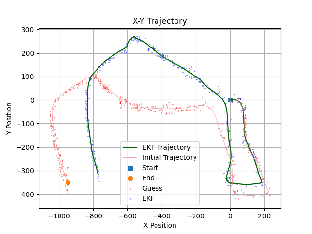
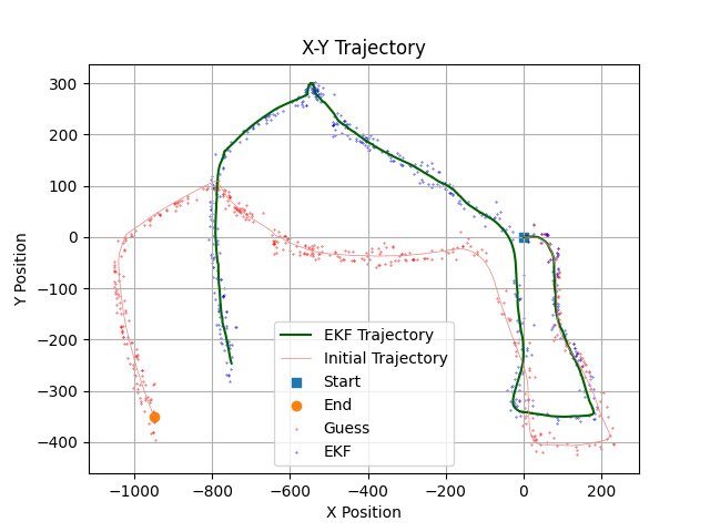
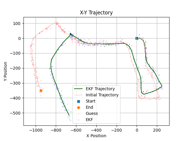
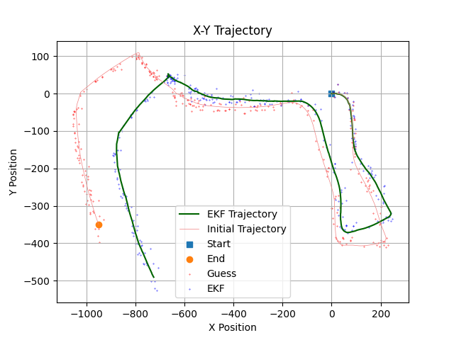
This section presents the trajectory and landmark positions after performing the complete visual-inertial SLAM with varying noise values.
The trajectories generated with varying noise values clearly illustrate the sensitivity of the estimated trajectory to factors such as the number of features utilized, map noise, and pixel noise. However, it appears that the number of feature points used has a greater effect on the estimated trajectory than either map noise or pixel noise. Determining the optimal trajectory becomes challenging without access to ground truth data or prior knowledge of the noise characteristics.
Theoretically, using more feature points should lead to a more accurate estimated trajectory. However, outliers, as well as poor or moving feature points, can significantly affect the trajectory estimation. Poorly selected feature points may not accurately represent the environment, leading to erroneous estimations. Similarly, moving feature points can introduce inconsistency in the data, as they are treated as static landmarks, causing inaccuracies in the trajectory estimation.
In conclusion, it is crucial to filter out poor feature points and accurately estimate noise parameters in visual-inertial SLAM to ensure robust performance and reliable estimation.


